What do sparse models do best?
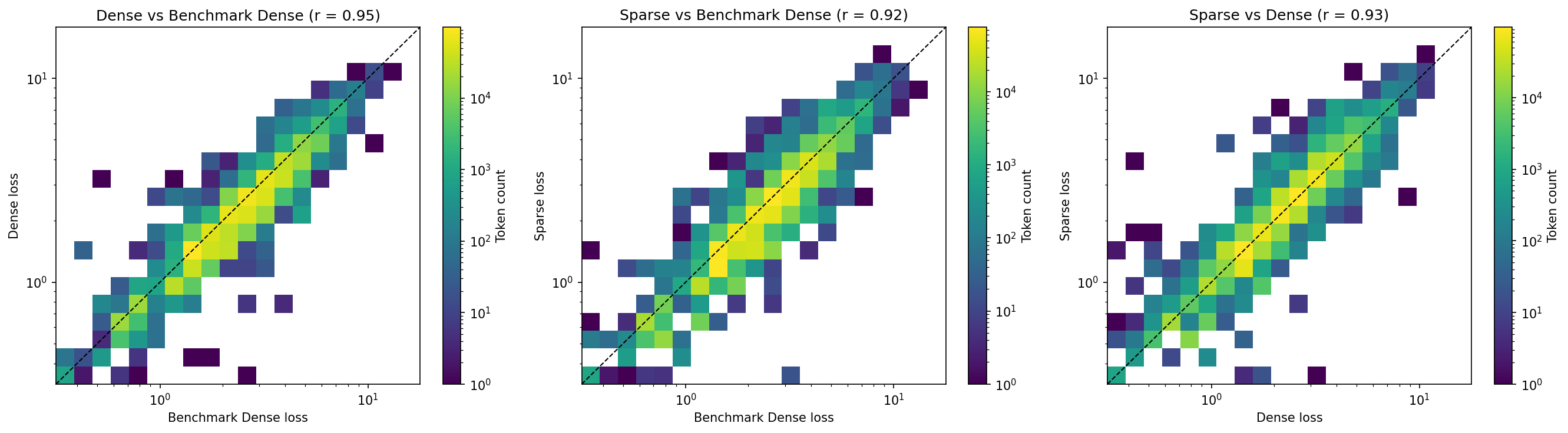
03 Jan 2026In a recent paper, the OpenAI interpretability team trained a series of transformers with sparse weights, and showed that the resulting models have interpretable circuits for certain tasks. In the Appendix, there is an experiment where they take one dense model, a second dense model trained with a different initialization, and a similarly capable sparse model, and compare the token-wise losses of the two dense models and the token-wise losses of the first dense model and the sparse model. They find that the correlation between the sparse model and dense model is nearly as high as the correlation between the two dense models, suggesting that the sparse model mostly fails on the same tokens as the dense model.
An important question for scaling sparse models is, What are the comparative advantages/disadvantages of sparse models, relative to similarly capable dense models? Can we characterize the instances where the sparse model excels and the dense model fails, and vice versa? This is a brief exploration of that question.
Setup
The circuit sparsity paper releases several pretrained models. We focus on three:
| Model | Our Label | Architecture | Average Loss |
|---|---|---|---|
dense1_1x |
Benchmark Dense | Standard dense transformer | 2.437 |
dense1_2x |
Dense | Dense transformer, 2x parameters | 2.200 |
csp_yolo1 |
Sparse | Weight-sparse transformer | 2.205 |
The dense and sparse model are roughly equal in capability (as measured by aggregate loss). Notably, the benchmark dense model is weaker. In Figure 33 of the paper, they create the benchmark model by retraining the dense model with a different initialization. I do not have the time or means to retrain another dense model, and for this investigation, the essential thing is that the sparse and dense model are similarly capable, so we use a weaker dense model as the benchmark.
For evaluation, I use the APPS dataset of Python coding problems. It consists of ~5,000 code samples. Some are truncated to fit in the model context window. The losses reported in the above table reflect the losses on this dataset.
Figure 33 reproduction
I start by reproducing Figure 33 and get similar results to the paper: The sparse and dense models have roughly similar correlations to the benchmark dense model.
Model divergence
We are interested in characterizing the off-diagonal tokens in the sparse-dense correlation grid: On which tokens does one model perform better than the other?
Key metric: ΔLoss
The metric we use to discuss this is ΔLoss, which is simply the difference in loss between the two models (usually on a single token, or group of tokens):
ΔLoss = Loss_Sparse − Loss_Dense
- ΔLoss < 0 → Sparse wins (lower loss is better)
- ΔLoss > 0 → Dense wins
- ΔLoss ≈ 0 → models perform similarly
Motivating hypothesis
Consider the question, On which tasks would we expect a sparse model to perform better than a dense model? An obvious (though a bit naive) answer is tasks that are better represented as sparse circuits. This helps us narrow the research question: What tasks are better represented as sparse circuits? One hypothesis is that tasks that are more deterministic are better represented as sparse circuits.
What do we mean by determinism?
Intuitively, a deterministic task is one where there is a single correct answer versus many correct answers. An arithmetic problem is deterministic, while a creative writing problem is not. We can try to formalize this by supposing there is an oracle model that perfectly models the pre-training distribution. Completions where the oracle model generates a low-entropy distribution are highly deterministic, high-entropy distributions are low determinism.
(Determinism is a bit of an overloaded term, and I don’t really mean to invoke definitions from other domains. Though they may be useful, ymmv.)
Token categorization
The first thing I did was ask Claude to group the most common tokens into meaningful categories, and show the difference in loss across each category. The results are below:
Key Findings
| Category | Count | Dense Loss | Sparse Loss | ΔLoss |
|---|---|---|---|---|
| Logical operators | 1,065 | 3.99 | 3.67 | -0.32 |
| Compound closing brackets | 40,456 | 2.09 | 1.88 | -0.21 |
| Digits | 50,986 | 1.76 | 1.67 | -0.09 |
| Closing brackets | 21,099 | 1.57 | 1.49 | -0.08 |
| Arithmetic operators | 35,272 | 2.58 | 2.53 | -0.05 |
| Opening brackets | 20,378 | 1.82 | 1.78 | -0.04 |
| Compound opening brackets | 51,920 | 2.27 | 2.23 | -0.04 |
| Punctuation | 73,478 | 1.73 | 1.71 | -0.03 |
| Indentation | 50,782 | 1.02 | 1.02 | -0.00 |
| Other | 320,398 | 2.35 | 2.37 | +0.01 |
| Common variable names | 81,789 | 2.47 | 2.50 | +0.03 |
| Comparison operators | 10,008 | 2.56 | 2.61 | +0.05 |
| Python keywords | 23,121 | 1.90 | 1.95 | +0.05 |
| Underscore patterns | 10,965 | 3.35 | 3.43 | +0.08 |
| Common builtins | 28,497 | 2.75 | 2.85 | +0.10 |
| Method calls | 8,692 | 2.65 | 2.82 | +0.18 |
| Control flow end | 7,742 | 2.06 | 2.28 | +0.22 |
| Multi-digit numbers | 8,451 | 4.13 | 4.39 | +0.26 |
| Control flow start | 25,045 | 2.50 | 2.85 | +0.35 |
The category results aren’t conclusive, but some items stick out:
- Sparse models are better at closing brackets, especially compound closing brackets. These are plausibly more deterministic tasks, on average.
- Dense models are better at control flow start/end and method calling. These are plausibly less deterministic tasks, on average.
Case study: closing brackets
Closing brackets are probably the best example of a highly deterministic task: The correct closing bracket sequence is perfectly determined by the opening sequence (though, there are potential contextual ambiguities, e.g., whether closing bracket sequences should be placed on a single line or across several lines).
One question we might have is whether sparse models do better as the closing bracket sequence becomes more complex. If sparse models are better at closing bracket completions because they are deterministic, then we might expect that advantage to be even more pronounced on hard versions of that task.
Below I show two tables. The first shows the difference in loss when predicting tokens that only have closing bracket characters (i.e., excluding colons, new lines, and other whitespace). The second shows the difference in loss over a larger set of closing bracket sequence (including colons, new lines, and other whitespace), aggregated over the number of closing brackets in the token.
Both are pretty straightforwardly interesting. In general, the advantage of the sparse model grows as the closing bracket sequence becomes longer.
| Token | Count | Dense Loss | Sparse Loss | ΔLoss |
|---|---|---|---|---|
)) |
1,811 | 2.64 | 2.18 | -0.47 |
]] |
474 | 3.29 | 2.94 | -0.35 |
]) |
1,512 | 2.30 | 2.07 | -0.23 |
)] |
464 | 2.71 | 2.53 | -0.17 |
} |
682 | 1.39 | 1.26 | -0.14 |
] |
10,691 | 1.57 | 1.47 | -0.09 |
) |
9,726 | 1.58 | 1.52 | -0.06 |
| Brackets | Tokens | Total Count | Avg ΔLoss |
|---|---|---|---|
| 3 | 1 | 183 | -0.71 |
| 2 | 17 | 10,151 | -0.40 |
| 1 | 41 | 50,605 | -0.11 |
Entropy as a measure of task determinism
Next I more directly invoke the use of entropy to measure task determinism. If the sparse model is better at highly deterministic tasks, then we might expect it to perform better on low-entropy completions.
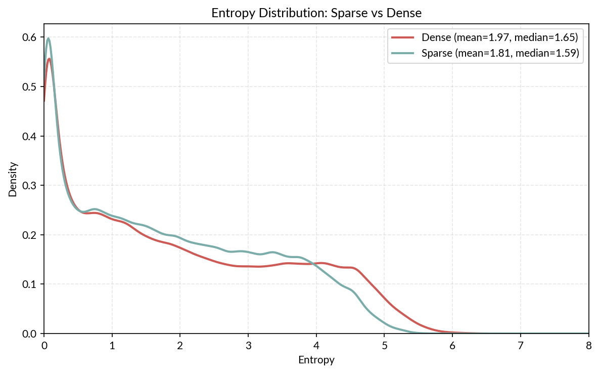
First we look at the subjective entropy distributions of each model over all completions. The below figure shows a density plot of each model’s entropy distribution (it was computed by differentiating a smoothed cumulative probability histogram). Notably, the sparse model has lower average entropy, and a slightly higher frequency of low (< 0.2) entropy predictions, though the difference is subtle.
When models diverge in confidence
It’s interesting that the sparse model is generally more confident than the dense model, but that doesn’t communicate much about the sorts of tasks the sparse model is better at. In addition to being more confident than the dense model, we might wonder whether the sparse model is better at being confident than the dense model.
The below table tries to answer the question: When one model is confident, and the other uncertain, how much better does the confident model perform? And how does this change depending on which model is the confident one?
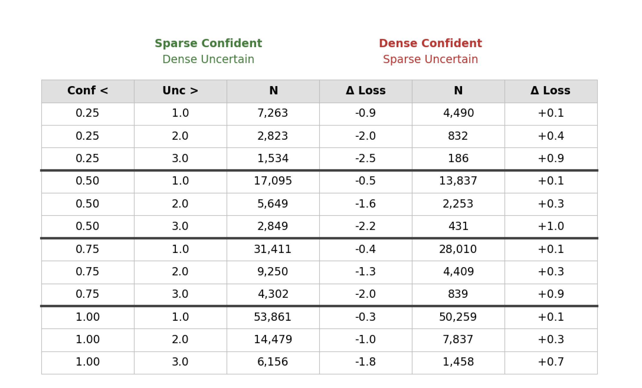
The effect is consistent: When the sparse model is confident and the dense model uncertain, its advantage is much larger than the dense model’s advantage when the situation is reversed. We might say that the confidence in the sparse model is a much stronger signal than confidence in the dense model. Further, it is much more common for the sparse model to be confident and the dense model uncertain than vice versa.
Oracle entropy analysis
The previous two analyses used the subjective entropy of each model. Here, lastly, we use a much more capable model (GPT-OSS 20B) to serve as our “oracle” model, classifying tokens as high- or low-entropy. Then we compute the loss of each model with respect to the entropy GPT-OSS assigned to that token.
I should note that GPT-OSS uses a different tokenizer than the sparse and dense models, so I had to do something a bit hacky: For each GPT-OSS token, we assign the entropy to every character in that token. Then, we compute entropy values for each sparse/dense token by taking the average entropy over each character in the span of that token.
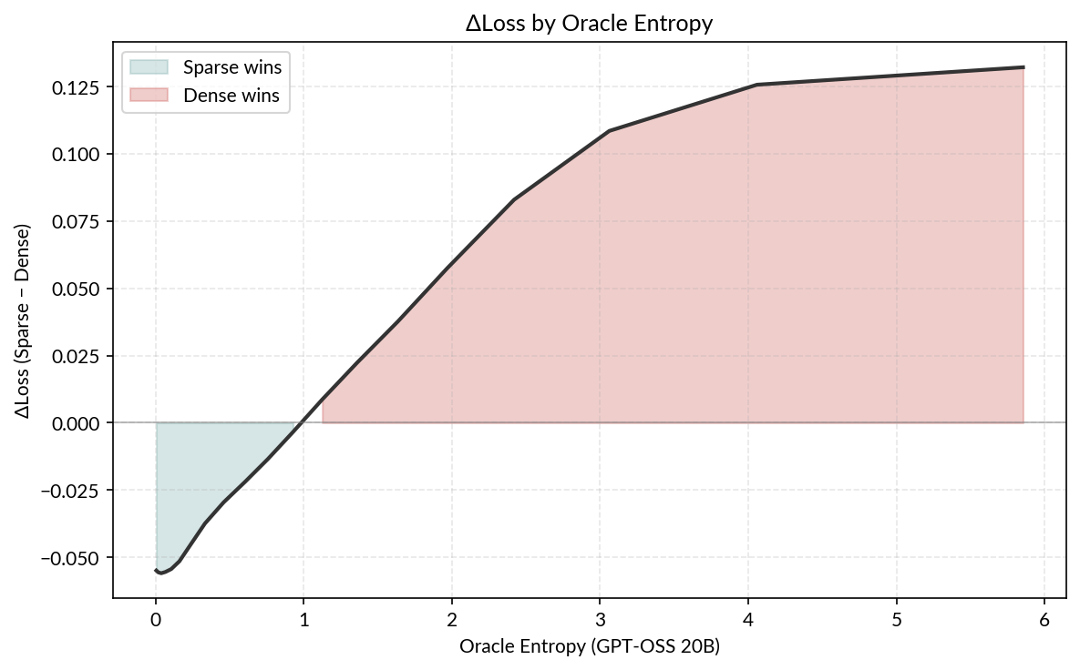
The trend is pretty strong! The advantage of the sparse model is strongest for low-entropy completions, and decreases as entropy increases.
Final thoughts
The epistemic status of these results are a bit shaky for a few reasons:
- The experiments here were pretty vibe-coded and need to be properly validated to constitute a rigorous analysis.
- I’m not performing any causal analyses, or even controlling for potentially confounding factors in any of the experiments. Some of the results could reflect spurious correlational artifacts.
- I arrived at the “sparse models better at deterministic tasks” hypothesis partly retrospectively, trying to explain some of the results shown here. My process was less “here is a hypothesis, let’s run these experiments to test it” and more “these results seem to point in this direction, let’s poke around more.”
So, I don’t want to make any particularly strong claims here. But at the minimum, this might be a useful lens for further exploration - I hope to engage more when I have time. If you want to pursue an ambitious vision for interpretability, it’s important not only to scale interpretable models to dense model capabilities, but to also characterize the relative strengths and weaknesses of interpretable models.